Dimensioning of IBPSA plug flow pipes for Vejle Nord LiveLab using Dymola FMI and Python

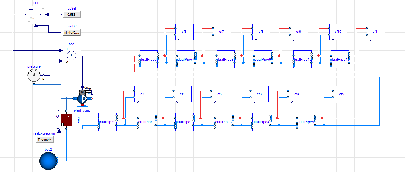
Usually district heating pipes are dimensioned based on the connected load which depends on the size of the houses and the domestic hot water usage. With houses becoming smarter and better in terms of insulation and general energy use, it seems interesting to rethink the dimensioning to be based on the consumption profiles. This can be done in Modelica through dynamic simulation of a district heating grid parts or the entire grid to consider hot water storage capacities which may be charged or discharged. One issue that arises with the predefined Modelica district heating components is that although the solvers are time-based, the parameters of installations cannot vary during the simulation. This issue is addressed in this case study where Modelica models are exported as FMUs and then the FMUs are simulated with multiple different input parameters being changed. Using this approach, it is possible for the researcher to choose which parameters to use to dimension pipes (known dimensioning tools use pressure drop gradient and volume speed) while keeping all other parameters fixed. Considered HVAC system consists of the IBPSA components (originating from IDEAS library): Dual pipe consisting of two PlugFlowPipe models, a heat exchanger and controlled underfloor heating.


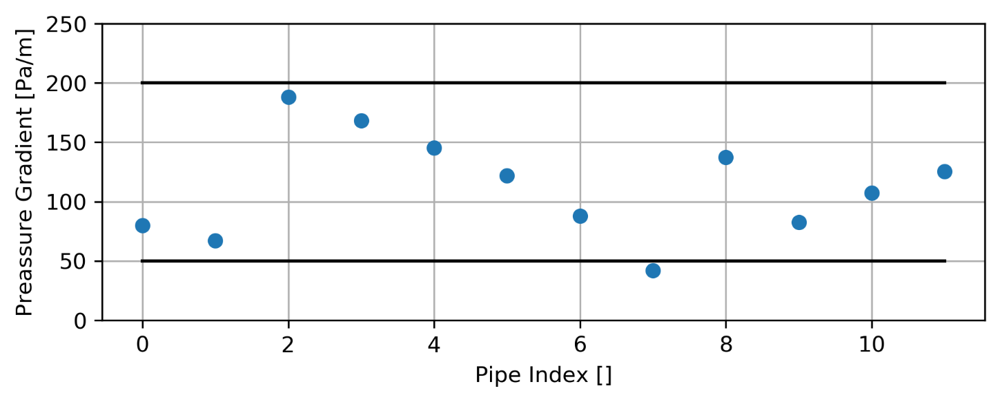
In the case study, it is shown how the pressure drop gradient is used with boundary values of 50 Pa/m and 200 Pa/m on a stretch of the road with 12 consumers with roughly estimated 15 – 70 m distances between them. The pressure gradient boundaries ensure that the investment cost for the pipes and the pumping work are kept within a realistic range. The exact size of the boundaries is set to match those used in Termis dimensioning tool which is one of the leading tools and widely used for pipe dimensioning. The pressure gradient boundaries ensure that the investment costs for the pipes and the pumping work are kept within a realistic scenario. The exact size of the boundaries is set to match those used in Termis, one of the leading tools for district heating calculations and widely used for pipe dimensioning. For this stretch of road in Vejle, the consumption profiles for the consumers are known and used to dimension the pipes. Pipes are dimensioned with a brute force algorithm testing of different pipes. The pipes sizes are obtained from a series of pipes from Isoplus. When looking at the results for the pressure gradient it is not possible for all pipes to have the exact same pressure gradient and, in some cases, a pipe that yields pressure gradients inside the boundaries might not be available in the pipe series. As shown in Fig.2, pipe number 7 has a pressure gradient outside the boundary values, here supervision of the algorithm is suggested since all pipe diameters yields pressure gradients outside boundary values for this location. The algorithm returns the pipe diameter with the pressure gradient which is lower than the lower boundary. These are first results obtained using the pipe dimensioning algorithm.

Factsheet

Thermal zoning

Number of buildings	12
Number of thermal zones (per building)	1
Complexity of thermal zone model	Low order
Coupling/Decoupling between district network and buildings	Decoupling

Tools

Simulation tool	Dymola / JModelica
Modelica libraries	IDEAS
Additional packages/workflows/scripts	PyFMI

Computational settings

Simulation time	3 days
Computational time	46 seconds for 4 iterations
Solver and tolerance	CVode / 1e-4(relative)
CPU speed	2.5 GHz