Appendix: Additional KPI Specification and Calculation
Summary
Advanced building controls are increasingly critical to achieve high energy efficiency, demand flexibility, and occupant comfort in buildings. However, large-scale adoption of emerging building control strategies requires verified performance. When performing verification, key performance indicators (KPIs) are necessary, which quantify performances of those building control strategies. Designing KPIs can be challenging, as they should not only capture how controls impacts the different aspects of building performance, but also enable fair comparison among different building control strategies under various operating conditions.
This appendix further elaborates on our efforts to design KPIs for simulation-based evaluation of building control strategies. In this appendix, we firstly introduce KPIs, including the motivation for having certain KPIs and how each KPI is calculated. We then discuss how those KPIs are integrated into the building emulators, which include building simulation models and necessary pre-and post-processing for performing simulation.
Acronyms and Abbreviations
Introduction
Key performance indicators (KPIs) for building control systems measure the behavior and impacts of such systems. Typically, a metric value from one controller is compared with a default criteria value or the same metric calculated from another controller (e.g., baseline). Such comparisons can quantify the pros and cons of a new controller or control system, which is a critical step in technology development. As summarized by [AJS14], common control performance indicators include energy, cost, peak load shifting capability, transient response, steady-state response, control of variables within bounds, reduction in fluctuations from a set-point, system efficiency, robustness to disturbances and changes, IAQ, thermal comfort, and computational time. These metrics were selectively used in previous studies. For example, [MQSX12] used energy usage as one of their KPIs, while [Hua11, MBDB10, PSFC11, RH11, XPC07, YP06] used metrics for control dynamic performance as qualitative evaluation. In this document, we attempted to answer two related questions:
What would be a comprehensive list of KPIs for control performance evaluation?
What are their definition and calculation formulas?
To answer the first question, we grouped KPIs into the following categories: energy-related, controller-related, system-related, disturbance-related, and occupant-related (as illustrated in the figure below). A building control system controls the HVAC system, which conditions the indoor space. The indoor space is occupied by people and has comfort demand. On the other side, the HVAC system needs energy, especially electricity, to operate. This demand links buildings to electric grids.
To answer the second question, we proposed methodologies to quantify KPIs in each category. Specifically, we discussed inputs for calculating each KPI and how those inputs are accessible in real buildings or emulators. We then provided detailed formulas to calculate each KPI based on those inputs.
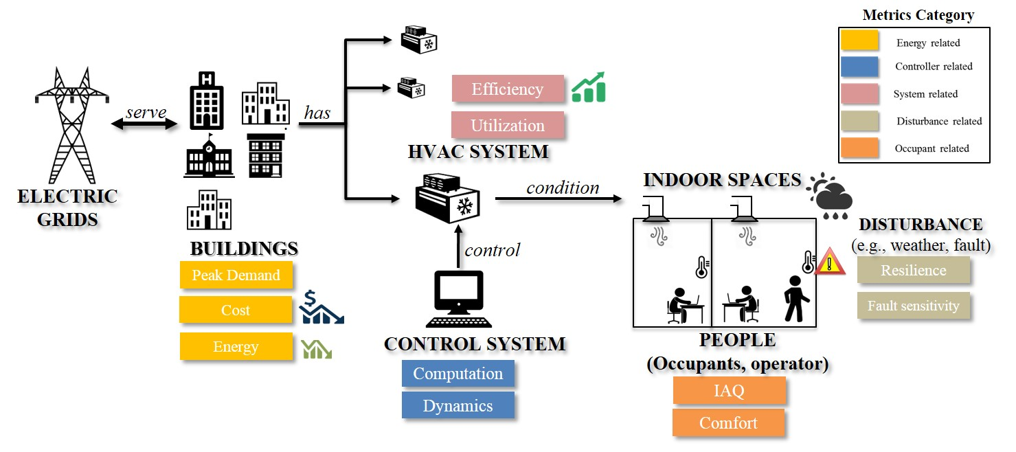
An overview of the conceptual design of control performance metrics
Description of Key Performance Indicators
Power demand metrics
Diversity factor is defined by the General Services Administration [GSA96] as the ratio of the sum of individual maximum demands to the maximum demand of the whole system:
(1)¶\[\dfrac{\sum_{e \in E}\max\limits_{{t_{0}}<t<{t_{1}}}{P_e(t_i)}}{\max\limits_{{t_{0}}<t<{t_{1}}}{\sum_{e \in E}P_e(t_i)}}\]Load factor can be expressed as follows based on the definition in [GSA96]:
(2)¶\[\dfrac{\overline{P_e(t_i)}}{\max\limits_{{t_{0}}<t<{t_{1}}}{P_e(t_i)}}\]Equipment power demand fraction at time \(t_i\) relative to total power demand at time \(t_i\), this can help rank the energy demand from equipment level:
(3)¶\[\dfrac{P_{e}(t_i)}{\sum_{e \in E}P_e(t_i)}\]Power peak demand during the period \([t_{0},t_{1}]\) :
(4)¶\[\max\limits_{{t_{0}}<t_i<{t_{1}}}{\sum_{e \in E}P_e(t_i)}\]
Energy usage metrics
Building energy usage has always been considered a key indicator of building performance. Energy usage refers to the fuels consumed by a building system at a given period. Such energy consumption can be further divided based on end-use type into multiple categories, i.e., space heating, cooling, ventilation, water heating, lighting, cooking, refrigeration, computing (including servers), office equipment, and other uses [Adm16]. Here, we listed energy consumption for equipment, total energy consumption, and combined the end-use energy usage into HVAC energy usage and non-HVAC energy usage.
Energy consumption of equipment \(e \in E\) during the period \([t_{0},t_{1}]\):
(5)¶\[\int_{t_i=t_{0}}^{t_{1}} P_e(t_i)dt\]Energy consumption fraction associated with equipment \(e\) during \([t_{0},t_{1}]\) :
(6)¶\[\dfrac{\int_{t_i=t_{0}}^{t_{1}}P_e(t_i)dt}{\sum_{e \in E}\int_{t_i=t_{0}}^{t_{1}}P_e(t_i)dt}\]Total building energy consumption during \([t_{0},t_{1}]\) :
(7)¶\[{\sum_{e \in E}\int_{t_i=t_{0}}^{t_{1}}P_e(t_i)dt}\]HVAC system energy consumption during \([t_{0},t_{1}]\) :
(8)¶\[{\sum_{e \in E}\int_{t_i=t_{0}}^{t_{1}}P_{e,AC}(t_i)dt}\]Non-HVAC system energy consumption during \([t_{0},t_{1}]\) :
(9)¶\[{\sum_{e \in E}\int_{t_i=t_{0}}^{t_{1}}P_e(t_i)dt}-{\sum_{e \in E}\int_{t_i=t_{0}}^{t_{1}}P_{e,AC}(t_i)dt}\]
Energy cost metrics
(10)¶\[{\sum_{e \in E}\int_{t_i=t_{0}}^{t_{1}}P_e(t_i)\lambda(t_i)dt}\]Let \(c_d(t_i)\) denote the fuel price (peak demand charge rate) at time \(t_i\). Considering the demand charge rate, [MQSX12] rewrote the cost metric as:
(11)¶\[{\sum_{e \in E}\int_{t_i=t_{0}}^{t_{1}}P_e(t_i)\lambda(t_i)dt}+\max\limits_{{t_{0}}<t<{t_{1}}}{\sum_{e \in E}\int_{t_i=t_{0}}^{t_{1}}P_e(t_i)\lambda_d(t_i)dt}\]
Thermal comfort metrics
Based on Fanger comfort model [Fan67, F+70], predicted percent of dissatisfied (\(PPD\)) people at each Predicted Mean Vote (\(PMV\)) can be calculated as:
(12)¶\[PPD = 100-95e^{-0.03353*PMV^4 - 0.2179*PMV^2}\]where \(PMV = (0.303e^{-0.036M}+0.028)(H-L)\); \(H\) is the internal heat production rate of an occupant per unit area (i.e., metabolic rate per unit area minus the rate of heat loss due to the performance of work, \(L\) is all the modes of energy loss from body )
Number of excursions outside of the comfort set for zone \(z\):
(13)¶\[|\{t_z ~|~ T_{t}^n \in S_c \land T_{t+1}^n \not\in S_c \}|\]Total time when the comfort indicator \(T\) is outside the comfort set \(S_c\) for zone \(z\), during the time interval \(\{t_{0},t_{1}\}\):
(14)¶\[t_{u,z} = \sum_{t_i=t_0}^{t_1}s(t_i)\]where \(s(t_i)=1\), if \(T^n_{t}\not \in S_c\), at time \(t_i\); \(s(t_i)=0\), if \(T^n_{t} \in S_c\), at time \(t_i\).
Total time when the comfort indicator \(T\) is outside the comfort set \(S_c\) for all the zones in the whole building \(z \in {Z}\), during the time interval \(\{t_{0},t_{1}\}\):
(15)¶\[t_{u,Z} = \sum_{z \in Z}\sum_{t_i=T_0}^{t_1}s(t_i)\]Percent time when the comfort indicator \(T\) is outside the comfort set \(S_c\) for zone \(z\), during the time interval See (16) \(\{t_{0},t_{1}\}\):
(16)¶\[\dfrac{|t_{u,z}|}{t_{1} - t_{0}}\]Maximum deviation from the comfort set for zone \(z\)
(17)¶\[max\{T^n_{min} - T_{l},T_{u} - T^n_{max}\}\]where \(T_{u} = \max\{T_t^n~|~T_t^n > T^n_{max}\}\) and \(T_{l} = \min\{T_t^n~|~T_t^n < T^n_{min}\}\).
System and equipment utilization metrics
period \([t_{0},t_{1}]\):
(18)¶\[\dfrac{1}{t_{1}-t_{0}}\sum_{t_i=t_{0}}^{t_{1}} O_{e}(i)\]Where \(O_{e}(i)=1\), if the equipment is ON, and \(O_{e}(i)=0\), if the equipment is OFF.
- The maximum capacity percentage of equipment \(e \in E\) during the period \([t_{0},t_{1}]\):(19)¶\[\dfrac{max\{C_{e, t} ~|~t \in \{t_{0},t_{1}\}\}}{C_{e,r}}\]
Where \(C_{e,r}\) is the rated maximum capacity of of equipment \(e \in E\) during the period \([t_{0},t_{1}]\).
The average capacity percentage of equipment \(e \in E\) during the period \([t_{0},t_{1}]\):
(20)¶\[\dfrac{average\{C_{e, t} ~|~t \in \{t_{0},t_{1}\}\}}{C_{e,r}}\]The average efficiency coefficient (e.g.,energy efficiency ratio, seasonal energy efficiency ratio, and coefficient of performance) of equipment \(e \in E\) during the period \([t_{0},t_{1}]\):
(21)¶\[{max\{\eta_{e, t} ~|~t \in \{t_{0},t_{1}\}\}}\]
Control dynamics metrics
Control performance assessment can be considered as an evaluation of the quality of control during normal and abnormal operation. It includes qualitative analysis (e.g., Bode plot, Nyquist plot) and quantitative evaluations (e.g., Harris index, mean of control error). Several studies have reviewed and compared the performance of those metrics [HSD99, Jel06, ONeillLW17]. Particularly, [ONeillLW17] compared the metrics for HVAC control loops and recommended the Harris index and VarBand because of their bounded values. Here we selected the Harris index as one metric. In addition, we added response speed, i.e., how fast the controller responds to a disturbance.
Let \(s_i\), \(M_i\), \(t_0\),\(t_1\), \(d_0\), and \(d_1\) denote the control setpoint for control variable \(i\), the actual measurement of this control variable \(i\), the time when a disturbance occurs, the time when the system re-balanced (actual measurement stays within \(\pm\) 10% of the setpoint), pre-disturbed value, and the disturbance value, respectively.
Based on [Har89], Harris index is calculated as follows:
(22)¶\[H=1-\frac{\delta^2_{mv}}{\delta^2_{y}}\]Where \(\delta^2_{mv}\) is the minimum variance of the control output obtained by maximum likelihood estimation method, and \(\delta^2_{y}\) is the variance of control outputs with respect to the setpoint.
Control response absolute speed:
(23)¶\[t_{0-1}=t_1-t_0\]Control response relative speed:
(24)¶\[\frac{t_{0-1}}{|d_1-d_0|}\]
Fault sensitivity metrics
Computation metrics
Controller prediction time at \(i^{th}\) iteration can be calculated as:
(26)¶\[t_p(i)=t_{p1}(i)-t_{p0}(i)\]Model simulation (or real building system operation) time length at \(i^{th}\) iteration can be calculated as:
(27)¶\[t_s(i)=t_{s1}(i)-t_{s0}(i)\]while total \(t_s(i)\) over a period of \([t_{0},t_{1}]\):
(28)¶\[t_s=\sum_{t_i=t_{0}}^{t_{1}}t_s(i)\]Real building system operation time length at \(i^{th}\) iteration can be calculated as:
(29)¶\[t_r(i)=t_{r1}(i)-t_{r0}(i)\]Total \(t_r\) over a period of \([t_{0},t_{1}]\) can be calculated as:
(30)¶\[t_r=\sum_{i=t_{0}}^{t_{1}}t_r(i)\]Total prediction-simulation time ratio:
(31)¶\[\frac{t_p}{t_s}\]Total modeling-operation time ratio:
(32)¶\[\frac{t_s}{t_r}\]
Air quality metrics
Average \(CO_2\) concentration for zone \(z\), during the period \([t_{0},t_{1}]\):
(33)¶\[\dfrac{1}{t_{1}-t_{0}}{\sum_{t_i=t_{0}}^{t_{1}}A_z(t_i)}\]Maximum \(CO_2\) concentration for zone \(z\), during the period \([t_{0},t_{1}]\):
(34)¶\[{max\{A_z(t_i) ~|~t_i \in \{t_{0},t_{1}\}\}}\]Total time when \(CO_2\) concentration \(A_z(t_i)\) is higher than the ASHRAE recommended value \(A_r\) for zone \(z\), during the time interval \(\{t_{0},t_{1}\}\):
(35)¶\[t(CO_2)_{u,z} = \sum_{t_i=T_0}^{T_z}s(t_i)\]where \(s(t_i)=1\), if \(A_z(t_i)\) \(>\) \(A_r\), at time \(t_i\); \(s(t_i)=0\), if \(A_z(t_i)\) \(\leq\) \(A_r\), at time \(t_i\).
Total time when \(CO_2\) concentration \(A_z(t_i)\) is higher than the ASHRAE recommended value \(A_r\) for all the zones in the whole building \(z \in {Z}\), during the time interval \(\{t_{0},t_{1}\}\):
(36)¶\[t(CO_2)_{u,Z} = \sum_{z \in Z}\sum_{t_i=T_0}^{T_z}s(t_i)\]where \(s(t_i)=1\), if \(A_z(t_i)\) \(>\) \(A_r\), at time \(t_i\); \(s(t_i)=0\), if \(A_z(t_i)\) \(\leq\) \(A_r\), at time \(t_i\).
Capability of the controller to steer flexibility
A controller capable of estimating and steering the flexibility available in a building supposes an added value, since it would be able to provide demand repsonse and ancillary services to the electric grid or district heating or cooling network. However, the explicit quantification of this KPI is particularly challenging because of the dependency of flexibility on the previous actions, current state, and various flexibility objectives that exist. For this reason, BOPTEST will utilize the operational cost KPI with dynamic pricing as a proxy for how the controller steers flexibility. Future work may specify dedicated tests and explicit quantification of flexibility.
KPI Implementation
KPI implementation refers to the process of calculating KPIs with predefined procedures, during or after the control evaluation. When performing simulation-based control evaluation, we streamline the KPI implementation by integrating the KPI calculation modules into the building emulators. Specifically, we categorize KPIs into two groups: Core KPI and customized KPI.
For KPIs in Core KPI, inputs for calculating them are tagged in the simulation model while the corresponding calculation methods are parts of the standard simulation process.
For KPIs in customized KPI, application programming interfaces are provided to allow users to specify the required inputs for calculating such KPIs and detailed calculation methods.
In the following subsections, we detail the implementation for the two groups, respectively.
Core KPI
Core KPI is intended to enable “apple-to-apple” comparisons among different building controls. To serve this purpose, KPIs in core KPI must be case insensitive, i.e., not depending on specific simulation case or simulation scenario. As of now, we consider two KPIs for key KPI: “HVAC system energy consumption”, as defined in (7), and “comfort”, as defined in (37).
where \({T_i}^k\) is the temperature of the \(i\)th zone at the discrete \(k\)th time step, \(T_{set}\) is the zone temperature set point, \({\Delta}t\) is the discrete time step length , \(M\) is the number of zones, and \(N\) is the number of discrete time steps.
Similarly, we rewrite Equation (7) into a discrete form, as shown below, to facilitate the calculation:
where \({P_{j}}^k\) is the power of the \(j\)th HVAC device at the discrete \(k\)th time step, \(S\) is the number of HVAC device.
In the Modelica building models, we specify the inputs for (37) and (38) with a module called IBPSA.Utilities.IO.SignalExchange.Read. This module allows users to define which variables are involved in a certain KPI calculation. For example, \({T_i}^k\) is defined with:
IBPSA.Utilities.IO.SignalExchange.Read TRooAir(KPIs=``comfort'',
y(unit=``K''),
Description=``Room air temperature''));
Likewise, \({P_{j}}^k\) is defined as:
IBPSA.Utilities.IO.SignalExchange.Read ETotHVAC(KPIs=``energy'',
y(unit=``J''),
Description=``Total HVAC energy''));
A Python script is created to extract this KPI related information into a dictionary as shown below:
{``energy'': [``ETotHVAC_y''],
``comfort'': [``TRooAir_y'']}
Then, the above dictionary is used to calculate the KPIs with the following Python module:
def get_kpis(self):
        ``Returns KPI data.

        Requires standard sensor signals.

        Parameters
        ----------
        None

        Returns
        kpis : dict
            Dictionary containing KPI names and values.
            {<kpi_name>:<kpi_value>}

        ''
        kpis = dict()
        # Calculate each KPI using json for signalsand save
        in dictionary
        for kpi in self.kpi_json.keys():
            print(kpi, type(kpi))
            if kpi == 'energy':
                # Calculate total energy [KWh - assumes measured
                in J]
                E = 0
                for signal in self.kpi_json[kpi]:
                    E = E + self.y_store[signal][-1]
                # Store result in dictionary
                kpis[kpi] = E*2.77778e-7 # Convert to kWh
            elif kpi == 'comfort':
                # Calculate total discomfort [K-h = assumes
                measured in K]
                tot_dis = 0
                heat_setpoint = 273.15+20
                for signal in self.kpi_json[kpi]:
                    data = np.array(self.y_store[signal])
                    dT_heating = heat_setpoint - data
                    dT_heating[dT_heating<0]=0
                    tot_dis = tot_dis + trapz(dT_heating,
                    self.y_store['time'])
                    /3600
                # Store result in dictionary
                kpis[kpi] = tot_dis

        return kpis
To summarize, the Core KPI is predefined at the building simulation model level and we don’t expect any modification from the control developers.
Customized KPI
The customized KPI is designed for those KPIs that are subject to certain control or building simulation models. Examples of those KPIs include controllable building power, which varies among different building simulation models.
To perform an analysis on the customized KPI, users must define the customized KPI with the following template:
``kpi1'':{
    ``name'': ``Average_power'',
    ``kpi_class'': ``MovingAve'',
    ``kpi_file'': ``kpi.kpi_example'',
    ``data_point_num'': 30,
    ``data_points'':
    {``x'':``PFan_y'',
     ``y'':``PCoo_y'',
     ``z'':``PHea_y'',
     ``s'':``PPum_y''
     }
}
The above definition actually contains two major parts:
The first part defines which module (in which file) calculates the corresponding KPI. In this example, the module for calculating the KPI \(Average\_power\) is the class \(MovingAve\) in the file \(kpi.kpi\_example\). It is noted that this module should contains one function called “calculation”, as shown below:
class MovingAve(object):
def __init__(self, config, **kwargs):
    self.name=config.get(``name'')

def calculation(self,data):
    return sum(data[``x''])/len(data[``x''])
The second part defines the inputs for calculating the KPIs. In this example, there are four inputs for calculating the KPI \(Average\_power\) and the sampling horizon length for those inputs is 30 minutes.
The user-defined information is then processed by the following Python module:
class cutomizedKPI(object):
    '''
      Class that implements the customized KPI calculation.
    '''
    def __init__(self, config, **kwargs):
        # import the KPI class based on the config files
        kpi_file=config.get(``kpi_file'')
        module = importlib.import_module(kpi_file)
        kpi_class = config.get(``kpi_class'')
        model_class = getattr(module, kpi_class)

        # instantiate the KPI calculation class
        self.model = model_class(config)
        # import data point mapping info
        self.data_points=config.get(``data_points'')
        # import the length of data array
        self.data_point_num=config.get(``data_point_num'')
        # initialize the data buffer
        self.data_buff=None

    # a function to process the streaming data
    def processing_data(self,data,num):
    # initialize the data arrays
        if self.data_buff is None:
           self.data_buff={}
           for point in self.data_points:
               self.data_buff[point]=[]
               self.data_buff[point].
    append(data[self.data_points[point]])
    # keep a moving window
        else:
           for point in self.data_points:
               self.data_buff[point].
           append(data[self.data_points[point]])
               if len(self.data_buff[point])>=num:
                    self.data_buff[point].pop(0)

    # a function to process the streaming data
    def calculation(self):
        res = self.model.calculation(self.data_buff)
        return res
The above module reads the KPI information, instantiates the KPI calculation class, and creates data buffers for the KPI calculation.
U.S. Energy Information Administration. 2012 commercial buildings energy consumption survey (cbecs) survey data. 2016.
Abdul Afram and Farrokh Janabi-Sharifi. Theory and applications of hvac control systems – a review of model predictive control (mpc). Building and Environment, 72(Supplement C):343–355, 2014. URL: http://www.sciencedirect.com/science/article/pii/S0360132313003363, doi:https://doi.org/10.1016/j.buildenv.2013.11.016.
ASHRAE. Ansi/ashrae standard 55-2010 thermal environmental conditions for human occupancy. 2010.
ASHRAE. Ashrae standard 62.1-2010 ventilation for acceptable indoor air quality. 2016.
Mesut Avci, Murat Erkoc, Amir Rahmani, and Shihab Asfour. Model predictive hvac load control in buildings using real-time electricity pricing. Energy and Buildings, 60(0):199–209, 2013. URL: http://www.sciencedirect.com/science/article/pii/S037877881300025X, doi:http://dx.doi.org/10.1016/j.enbuild.2013.01.008.
Yan Chen, Sen Huang, and Draguna Vrabie. A simulation based approach for impact assessment of physical faults: large commercial building hvac case study. 2018 Building Performance Analysis Conference and SimBuild co-organized by ASHRAE and IBPSA-USA, September 26-28, Chicago, IL 2018.
Velimir Congradac and Filip Kulic. Hvac system optimization with co2 concentration control using genetic algorithms. Energy and Buildings, 41(5):571–577, 2009. URL: http://www.sciencedirect.com/science/article/pii/S0378778808002685, doi:http://dx.doi.org/10.1016/j.enbuild.2008.12.004.
PO Fanger. Calculation of thermal comfort, introduction of a basic comfort equation. ASHRAE transactions, 73:III–4, 1967.
Poul O Fanger and others. Thermal comfort. analysis and applications in environmental engineering. Thermal comfort. Analysis and applications in environmental engineering., 1970.
GSA. Federal standard 1037c telecommunications: glossary of telecommunication terms. 1996. URL: https://www.its.bldrdoc.gov/fs-1037/fs-1037c.htm.
T. J. Harris. Assessment of control loop performance. Canadian Journal of Chemical Engineering, 67(5):856–861, 1989. URL: <Go to ISI>://A1989CA59200019.
T. J. Harris, C. T. Seppala, and L. D. Desborough. A review of performance monitoring and assessment techniques for univariate and multivariate control systems. Journal of Process Control, 9(1):1–17, 1999. URL: <Go to ISI>://WOS:000078128300001, doi:Doi 10.1016/S0959-1524(98)00031-6.
Gongsheng Huang. Model predictive control of vav zone thermal systems concerning bi-linearity and gain nonlinearity. Control Engineering Practice, 19(7):700–710, 2011. URL: http://www.sciencedirect.com/science/article/pii/S0967066111000451, doi:https://doi.org/10.1016/j.conengprac.2011.03.005.
M. Jelali. An overview of control performance assessment technology and industrial applications. Control Engineering Practice, 14(5):441–466, 2006. URL: <Go to ISI>://WOS:000236459500001, doi:10.1016/j.conengprac.2005.11.005.
Jingran Ma, Joe Qin, Timothy Salsbury, and Peng Xu. Demand reduction in building energy systems based on economic model predictive control. Chemical Engineering Science, 67(1):92–100, 2012. URL: http://www.sciencedirect.com/science/article/pii/S0009250911005240, doi:https://doi.org/10.1016/j.ces.2011.07.052.
Peter May-Ostendorp, Gregor P Henze, Charles D Corbin, Balaji Rajagopalan, and Clemens Felsmann. Model-predictive control of mixed-mode buildings with rule extraction. Building and Environment, 46(2):428–437, 2011.
Petru-Daniel Moroşan, Romain Bourdais, Didier Dumur, and Jean Buisson. Building temperature regulation using a distributed model predictive control. Energy and Buildings, 42(9):1445–1452, 2010. URL: http://www.sciencedirect.com/science/article/pii/S0378778810000915, doi:10.1016/j.enbuild.2010.03.014.
Nabil Nassif. A robust co2-based demand-controlled ventilation control strategy for multi-zone hvac systems. Energy and Buildings, 45(0):72–81, 2012. URL: http://www.sciencedirect.com/science/article/pii/S0378778811004622, doi:http://dx.doi.org/10.1016/j.enbuild.2011.10.018.
Z. O'Neill, Y. F. Li, and K. Williams. Hvac control loop performance assessment: a critical review (1587-rp). Science and Technology for the Built Environment, 23(4):619–636, 2017. URL: <Go to ISI>://WOS:000400981400008, doi:10.1080/23744731.2016.1239466.
Frauke Oldewurtel, Alessandra Parisio, Colin N Jones, Dimitrios Gyalistras, Markus Gwerder, Vanessa Stauch, Beat Lehmann, and Manfred Morari. Use of model predictive control and weather forecasts for energy efficient building climate control. Energy and Buildings, 45:15–27, 2012.
Samuel Prívara, Jan Široký, Lukáš Ferkl, and Jiří Cigler. Model predictive control of a building heating system: the first experience. Energy and Buildings, 43(2):564–572, 2011. URL: http://www.sciencedirect.com/science/article/pii/S0378778810003749, doi:https://doi.org/10.1016/j.enbuild.2010.10.022.
J. Rehrl and M. Horn. Temperature control for hvac systems based on exact linearization and model predictive control. In IEEE International Conference on Control Applications (CCA), 1119–1124. 2011. doi:10.1109/CCA.2011.6044437.
Zhongwei Sun, Shengwei Wang, and Zhenjun Ma. In-situ implementation and validation of a co2-based adaptive demand-controlled ventilation strategy in a multi-zone office building. Building and Environment, 46(1):124–133, 2011. URL: http://www.sciencedirect.com/science/article/pii/S0360132310002131, doi:http://dx.doi.org/10.1016/j.buildenv.2010.07.008.
J. Sundell. On the history of indoor air quality and health. Indoor Air, 14:51–58, 2004. URL: <Go to ISI>://WOS:000223590700007, doi:10.1111/j.1600-0668.2004.00273.x.
J. Sundell, H. Levin, W. W. Nazaroff, W. S. Cain, W. J. Fisk, D. T. Grimsrud, F. Gyntelberg, Y. Li, A. K. Persily, A. C. Pickering, J. M. Samet, J. D. Spengler, S. T. Taylor, and C. J. Weschler. Ventilation rates and health: multidisciplinary review of the scientific literature. Indoor Air, 21(3):191–204, 2011. URL: <Go to ISI>://WOS:000290490300004, doi:10.1111/j.1600-0668.2010.00703.x.
Xue-Cheng Xi, Aun-Neow Poo, and Siaw-Kiang Chou. Support vector regression model predictive control on a hvac plant. Control Engineering Practice, 15(8):897–908, 2007. URL: http://www.sciencedirect.com/science/article/pii/S0967066106001766, doi:https://doi.org/10.1016/j.conengprac.2006.10.010.
Shui Yuan and Ronald Perez. Multiple-zone ventilation and temperature control of a single-duct vav system using model predictive strategy. Energy and Buildings, 38(10):1248–1261, 2006. URL: http://www.sciencedirect.com/science/article/pii/S0378778806000764, doi:https://doi.org/10.1016/j.enbuild.2006.03.007.