Buildings.Examples.VAVReheat.ASHRAE2006.
with the addition of CO2 concentration tracking,
variable efficiency heat pump model, variable efficiency chiller model,
and BOPTEST signal exchange blocks. The emphasis is on the control of
the air distribution system and not on the control of the
central plant equipment providing
hot and chilled water to the distribution system.
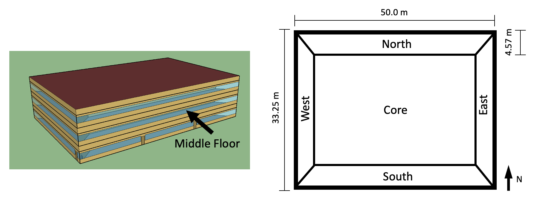
The test case represents the middle floor of an office building located in Chicago, IL, as described in the set of DOE Commercial Building Benchmarks for new construction (Deru et al, 2009) and shown in the figure below. The represented floor has five zones, with four perimeter zones and one core zone. Each perimeter zone has a window-to-wall ratio of 0.33. The height of each zone is 2.74 m and the areas are as follows:
The upper and lower boundaries of the zones (top of zone air volume and bottom of 0.1 m floor concrete slab) assume the corresponding zones of the floor above and the floor below are at the same conditions as the middle floor. Therefore, the roof and the ground floor with exposure to ambient conditions are not explicitly modeled. The zones on the floor are assumed to be paritioned by internal walls with 10 m by 2.1 m openings, through which air is exchanged.
Deru M., K. Field, D. Studer, K. Benne, B. Griffith, P. Torcellini, M. Halverson, D. Winiarski, B. Liu, M. Rosenberg, J. Huang, M. Yazdanian, and D. Crawley. DOE commercial building research benchmarks for commercial buildings. Technical report, U.S. Department of Energy, Energy Efficiency and Renewable Energy, Office of Building Technologies, Washington, DC, 2009.
The envelope thermal properties meet ASHRAE Standard 90.1-2004.
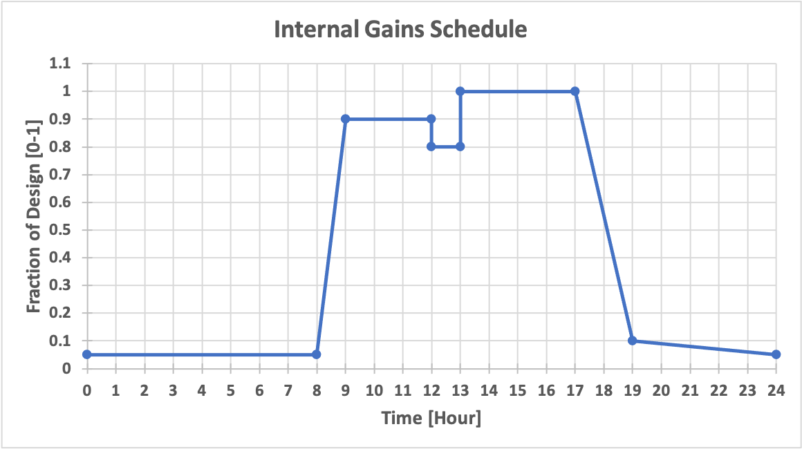
The design occupancy density is 0.05 people/m2. The number of occupants present in each zone at any time coincides with the internal gain schedule defined in the next section. The occupied time for the HVAC system is between 6 AM and 7 PM each day. The unoccupied time is outside of this period.
The design internal gains including lighting, plug loads, and people are combined 20 W/m2 with a radiant-convective-latent split of 40%-40%-20%. The internal gains are activated according to the schedule in the figure below.
The weather data is from TMY3 for Chicago O'Hare International Airport.
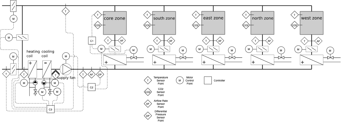
The HVAC system is a multi-zone single-duct Variable Air Volume (VAV) system with pressure-independent terminal boxes with reheat. A schematic of the system is shown in the figure below. The cooling and heating coils are water-based served by an air-cooled chiller and air-to-water heat pump respectively. The available sensor and control points, marked on the figure below and described in more detail in the Section Model IO's, are those specified as required by ASHRAE Guideline 36 2018 Section 4 List of Hardwired Points, specifically Table 4.2 VAV Terminal Unit with Reheat and Table 4.6 Multiplie-Zone VAV Air Handling Unit, as well as some that are specified as application specific or optional.
The terminal box dampers have exponential opening characteristics with design airflow rates defined in the table below. The design system airflow rate includes a 0.7 load diversity factor and is defined in the table below. The minimum outside airflow for each zone is calculated using outside airflow rates of 0.3e-3 m3/s-m2 and 2.5e-3 m3/s-person. The limiting zone air distribution effectiveness is 0.8 and the occupant diversity ratio is 0.7. This leads to the minimum outside airflow rates for each zone and system defined in the table below.
Table 1: Zone Terminal Unit and System Specifications Summary
| Name | Design Airflow [m3/s] | Min OA Airflow [m3/s] | Design Heating Load [kW] |
|---|---|---|---|
| North | 0.947948667 | 0.1102769 | 6.87 |
| South | 0.947948667 | 0.1102769 | 6.87 |
| East | 0.9001996 | 0.0698148 | 6.52 |
| West | 0.700155244 | 0.0698148 | 5.07 |
| Core | 4.4966688 | 0.5231070 | 32.6 |
| System | 5.595044684 | 0.8590431 |
The supply fan hydraulic efficiency is constant at 0.7 and the motor efficiency is constant at 0.7. The cooling coil is served by an air-cooled chiller supplying 6 degC water with varying COP according to a York YCAL0033EE chiller as modeled by the ElectricEIR model with coefficients defined in EnergyPlus v9.4.0. The peak design load on the chiller is 101 kW, equal to the design load on the cooling coil. A chilled water distribution pump circulates water from the chiller with a design head of 45 kPa and design mass flow equal to that of the chiller of 4.3 kg/s. The heating coil and terminal box reheat coils are served by a single air-to-water heat pump supplying 45 degC water with varying COP as 0.3 of the carnot COP. The peak design load on the heat pump is 122 kW, equal to sum of design loads on the heating coil in the AHU plus zone terminal box reheat coils multiplied by a load diversity factor of 0.85. A hot water distribution pump circulates water from the heat pump with a design head of 45 kPa and design mass flow equal to that of the heat pump of 2.9 kg/s.
The baseline control emulates a typical scheme seen in practice and is based on
the ASHRAE VAV 2A2-21232 of the Sequences of Operation for Common HVAC Systems 2006
as well as that which is implemented as baseline control in the Modelica Buildings
Library model
Buildings.Examples.VAVReheat.ASHRAE2006.
Setpoints and equipment enable/disable are determined by a schedule-based supervisory control
scheme that defines a set of operating modes. This scheme is summarized in
Table 2 below. An addition is made in this implementation from the one in Modelica Buildings Library
to add an Unoccupied Night Set Up mode, which allows for the system turning on
during unoccupied hours to maintain a cooling set point.
Table 2: HVAC Operating Mode Summary
| Name | Condition | TZonHeaSet [degC] | TZonCooSet [degC] | Fan [degC] | TSupSet [degC] | Economizer | Min OA Flow |
|---|---|---|---|---|---|---|---|
| Occupied | In occupied period. | 20 | 24 | Enabled | 12 | Enabled | Ventilation |
| Unoccupied off | In unoccupied period, all TZon within setback deadband. Minimum state time is 1 min. | 12 | 30 | Disabled | 12 | Disabled | Zero |
| Unoccupied, night setback | In unoccupied period, minimum TZon below unoccupied TZonHeaSet. Minimum state time is 30 min. | 12 | 30 | Enabled | 35 | Disabled | Zero |
| Unoccupied, night setup | In unoccupied period, maximum TZon above unoccupied TZonCooSet. Minimum state time is 30 min. | 12 | 30 | Enabled | 35 | Enabled | Zero |
| Unoccupied, warm-up | In unoccupied period, within 30 minutes of occupied period, average TZon below occupied TZonHeaSet | 20 | 30 | Enabled | 35 | Disabled | Zero |
| Unoccupied, pre-cool | In unoccupied period, within 30 minutes of occupied period, outside TDryBul below limit of 13 degC, average TZon above occupied TZonCooSet | 12 | 24 | Enabled | 12 | Enabled | Zero |
Once the operating mode is determined, a number of low-level, local-loop controllers are used to maintain the desired setpoints using the available actuators. The primary local-loop controllers are specified on the diagram above as C1 to C3.
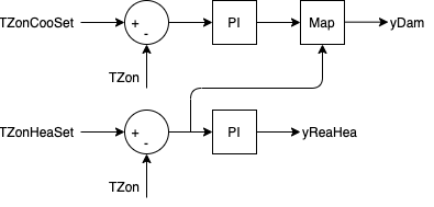
C1 is responsible for maintaining the zone temperature setpoints as determined by the operating mode of the system and implements dual-maximum logic, as shown in the Figure below. It takes as inputs the zone temperature heating and cooling setpoints and zone temperature measurement, and outputs the desired airflow rate of the damper and position of the reheat valve. Seperate PI controllers (both k = 0.1 and Ti = 120 s) are used for control of the damper airflow for cooling and reheat valve position for heating. If the zone requires heating, the desired airflow rate of the damper is mapped to the specified maximum value for heating.
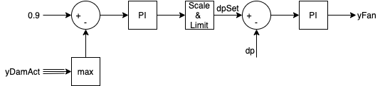
C2 is responsible for maintaining the duct static pressure setpoint and implements a duct static pressure reset strategy. The first step of the controller takes as input all of the terminal box damper positions and outputs a duct static pressure setpoint using a PI controller (k = 0.1 and Ti = 60 s) such that the maximum damper position is maintained at 0.9. The second step then maintains this setpoint using a PI controller (k = 0.5 and Ti = 15 s) and measured duct static pressure as input to output a fan speed setpoint.
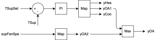
C3 is responsible for maintaining the supply air temperature setpoint as well as the minimum outside air flow rate as determined by the operating mode of the system. It takes as inputs the supply air temperature setpoint, supply air temperature measurement, outside drybulb temperature measurement, and supply fan speed. The first part of the controller uses a PI controller (k = 0.01, Ti = 120 s) for supply air temperature setpoint tracking to output a signal that is then mapped to position setpoints for the heating coil valve, cooling coil valve, and outside air damper position. If the heating valve is commanded to open and the supply fan is determined to be enabled (either by schedule or by supply air flow detection of at least 5% design air flow), the heating coil pump is enabled. Similar for cooling coil. The second part of the controller uses a map to determine the minimum outside air damper position for the given fan speed to provide minimum outside air requirements. Interpolation points for the map are assumed to be provided during commissioning and are given as follows. For a fan speed of 0.44, the minimum outside air damper position is 0.47. For a fan speed of 1.0, the minimum position is 0.32. The maximum of the two outside air damper position signals is finally output to ensure at least enough enough airflow is delivered for ventilation when needed. The economizer is enabled only if the outside drybulb temperature is lower than the return air temperature.
Also present, but not depicted in the diagrams above, is a freeze stat controller. This controller detects potentially freezing conditions by measuring the mixed air temperature and determining if it is less than a limit, 3 degC. If true, the controller will fully open the heating coil valve and enable the heating coil pump.
hvac_oveAhu_TSupSet_activate [1] [min=0, max=1]: Activation signal to overwrite input hvac_oveAhu_TSupSet_u where 1 activates, 0 deactivates (default value)
hvac_oveAhu_TSupSet_u [K] [min=285.15, max=313.15]: Supply air temperature setpoint for AHU
hvac_oveAhu_dpSet_activate [1] [min=0, max=1]: Activation signal to overwrite input hvac_oveAhu_dpSet_u where 1 activates, 0 deactivates (default value)
hvac_oveAhu_dpSet_u [Pa] [min=50.0, max=410.0]: Supply duct pressure setpoint for AHU
hvac_oveAhu_yCoo_activate [1] [min=0, max=1]: Activation signal to overwrite input hvac_oveAhu_yCoo_u where 1 activates, 0 deactivates (default value)
hvac_oveAhu_yCoo_u [1] [min=0.0, max=1.0]: Cooling coil valve control signal for AHU
hvac_oveAhu_yFan_activate [1] [min=0, max=1]: Activation signal to overwrite input hvac_oveAhu_yFan_u where 1 activates, 0 deactivates (default value)
hvac_oveAhu_yFan_u [1] [min=0.0, max=1.0]: Supply fan speed setpoint for AHU
hvac_oveAhu_yHea_activate [1] [min=0, max=1]: Activation signal to overwrite input hvac_oveAhu_yHea_u where 1 activates, 0 deactivates (default value)
hvac_oveAhu_yHea_u [1] [min=0.0, max=1.0]: Heating coil valve control signal for AHU
hvac_oveAhu_yOA_activate [1] [min=0, max=1]: Activation signal to overwrite input hvac_oveAhu_yOA_u where 1 activates, 0 deactivates (default value)
hvac_oveAhu_yOA_u [1] [min=0.0, max=1.0]: Outside air damper position setpoint for AHU
hvac_oveAhu_yPumCoo_activate [1] [min=0, max=1]: Activation signal to overwrite input hvac_oveAhu_yPumCoo_u where 1 activates, 0 deactivates (default value)
hvac_oveAhu_yPumCoo_u [1] [min=0.0, max=1.0]: Cooling coil pump control signal for AHU
hvac_oveAhu_yPumHea_activate [1] [min=0, max=1]: Activation signal to overwrite input hvac_oveAhu_yPumHea_u where 1 activates, 0 deactivates (default value)
hvac_oveAhu_yPumHea_u [1] [min=0.0, max=1.0]: Heating coil pump control signal for AHU
hvac_oveAhu_yRet_activate [1] [min=0, max=1]: Activation signal to overwrite input hvac_oveAhu_yRet_u where 1 activates, 0 deactivates (default value)
hvac_oveAhu_yRet_u [1] [min=0.0, max=1.0]: Return air damper position setpoint for AHU
hvac_oveZonActCor_yDam_activate [1] [min=0, max=1]: Activation signal to overwrite input hvac_oveZonActCor_yDam_u where 1 activates, 0 deactivates (default value)
hvac_oveZonActCor_yDam_u [1] [min=0.0, max=1.0]: Damper position setpoint for zone cor
hvac_oveZonActCor_yReaHea_activate [1] [min=0, max=1]: Activation signal to overwrite input hvac_oveZonActCor_yReaHea_u where 1 activates, 0 deactivates (default value)
hvac_oveZonActCor_yReaHea_u [1] [min=0.0, max=1.0]: Reheat control signal for zone cor
hvac_oveZonActEas_yDam_activate [1] [min=0, max=1]: Activation signal to overwrite input hvac_oveZonActEas_yDam_u where 1 activates, 0 deactivates (default value)
hvac_oveZonActEas_yDam_u [1] [min=0.0, max=1.0]: Damper position setpoint for zone eas
hvac_oveZonActEas_yReaHea_activate [1] [min=0, max=1]: Activation signal to overwrite input hvac_oveZonActEas_yReaHea_u where 1 activates, 0 deactivates (default value)
hvac_oveZonActEas_yReaHea_u [1] [min=0.0, max=1.0]: Reheat control signal for zone eas
hvac_oveZonActNor_yDam_activate [1] [min=0, max=1]: Activation signal to overwrite input hvac_oveZonActNor_yDam_u where 1 activates, 0 deactivates (default value)
hvac_oveZonActNor_yDam_u [1] [min=0.0, max=1.0]: Damper position setpoint for zone nor
hvac_oveZonActNor_yReaHea_activate [1] [min=0, max=1]: Activation signal to overwrite input hvac_oveZonActNor_yReaHea_u where 1 activates, 0 deactivates (default value)
hvac_oveZonActNor_yReaHea_u [1] [min=0.0, max=1.0]: Reheat control signal for zone nor
hvac_oveZonActSou_yDam_activate [1] [min=0, max=1]: Activation signal to overwrite input hvac_oveZonActSou_yDam_u where 1 activates, 0 deactivates (default value)
hvac_oveZonActSou_yDam_u [1] [min=0.0, max=1.0]: Damper position setpoint for zone sou
hvac_oveZonActSou_yReaHea_activate [1] [min=0, max=1]: Activation signal to overwrite input hvac_oveZonActSou_yReaHea_u where 1 activates, 0 deactivates (default value)
hvac_oveZonActSou_yReaHea_u [1] [min=0.0, max=1.0]: Reheat control signal for zone sou
hvac_oveZonActWes_yDam_activate [1] [min=0, max=1]: Activation signal to overwrite input hvac_oveZonActWes_yDam_u where 1 activates, 0 deactivates (default value)
hvac_oveZonActWes_yDam_u [1] [min=0.0, max=1.0]: Damper position setpoint for zone wes
hvac_oveZonActWes_yReaHea_activate [1] [min=0, max=1]: Activation signal to overwrite input hvac_oveZonActWes_yReaHea_u where 1 activates, 0 deactivates (default value)
hvac_oveZonActWes_yReaHea_u [1] [min=0.0, max=1.0]: Reheat control signal for zone wes
hvac_oveZonSupCor_TZonCooSet_activate [1] [min=0, max=1]: Activation signal to overwrite input hvac_oveZonSupCor_TZonCooSet_u where 1 activates, 0 deactivates (default value)
hvac_oveZonSupCor_TZonCooSet_u [K] [min=285.15, max=313.15]: Zone air temperature cooling setpoint for zone cor
hvac_oveZonSupCor_TZonHeaSet_activate [1] [min=0, max=1]: Activation signal to overwrite input hvac_oveZonSupCor_TZonHeaSet_u where 1 activates, 0 deactivates (default value)
hvac_oveZonSupCor_TZonHeaSet_u [K] [min=285.15, max=313.15]: Zone air temperature heating setpoint for zone cor
hvac_oveZonSupEas_TZonCooSet_activate [1] [min=0, max=1]: Activation signal to overwrite input hvac_oveZonSupEas_TZonCooSet_u where 1 activates, 0 deactivates (default value)
hvac_oveZonSupEas_TZonCooSet_u [K] [min=285.15, max=313.15]: Zone air temperature cooling setpoint for zone eas
hvac_oveZonSupEas_TZonHeaSet_activate [1] [min=0, max=1]: Activation signal to overwrite input hvac_oveZonSupEas_TZonHeaSet_u where 1 activates, 0 deactivates (default value)
hvac_oveZonSupEas_TZonHeaSet_u [K] [min=285.15, max=313.15]: Zone air temperature heating setpoint for zone eas
hvac_oveZonSupNor_TZonCooSet_activate [1] [min=0, max=1]: Activation signal to overwrite input hvac_oveZonSupNor_TZonCooSet_u where 1 activates, 0 deactivates (default value)
hvac_oveZonSupNor_TZonCooSet_u [K] [min=285.15, max=313.15]: Zone air temperature cooling setpoint for zone nor
hvac_oveZonSupNor_TZonHeaSet_activate [1] [min=0, max=1]: Activation signal to overwrite input hvac_oveZonSupNor_TZonHeaSet_u where 1 activates, 0 deactivates (default value)
hvac_oveZonSupNor_TZonHeaSet_u [K] [min=285.15, max=313.15]: Zone air temperature heating setpoint for zone nor
hvac_oveZonSupSou_TZonCooSet_activate [1] [min=0, max=1]: Activation signal to overwrite input hvac_oveZonSupSou_TZonCooSet_u where 1 activates, 0 deactivates (default value)
hvac_oveZonSupSou_TZonCooSet_u [K] [min=285.15, max=313.15]: Zone air temperature cooling setpoint for zone sou
hvac_oveZonSupSou_TZonHeaSet_activate [1] [min=0, max=1]: Activation signal to overwrite input hvac_oveZonSupSou_TZonHeaSet_u where 1 activates, 0 deactivates (default value)
hvac_oveZonSupSou_TZonHeaSet_u [K] [min=285.15, max=313.15]: Zone air temperature heating setpoint for zone sou
hvac_oveZonSupWes_TZonCooSet_activate [1] [min=0, max=1]: Activation signal to overwrite input hvac_oveZonSupWes_TZonCooSet_u where 1 activates, 0 deactivates (default value)
hvac_oveZonSupWes_TZonCooSet_u [K] [min=285.15, max=313.15]: Zone air temperature cooling setpoint for zone wes
hvac_oveZonSupWes_TZonHeaSet_activate [1] [min=0, max=1]: Activation signal to overwrite input hvac_oveZonSupWes_TZonHeaSet_u where 1 activates, 0 deactivates (default value)
hvac_oveZonSupWes_TZonHeaSet_u [K] [min=285.15, max=313.15]: Zone air temperature heating setpoint for zone wes
chi_reaFloSup_y [m3/s] [min=None, max=None]: Supply water flow rate of chiller
chi_reaPChi_y [W] [min=None, max=None]: Electric power consumed by chiller
chi_reaPPumDis_y [W] [min=None, max=None]: Electric power consumed by chilled water distribution pump
chi_reaTRet_y [K] [min=None, max=None]: Return water temperature of chiller
chi_reaTSup_y [K] [min=None, max=None]: Supply water temperature of chiller
heaPum_reaFloSup_y [m3/s] [min=None, max=None]: Supply water flow rate of heat pump
heaPum_reaPHeaPum_y [W] [min=None, max=None]: Electric power consumed by heat pump
heaPum_reaPPumDis_y [W] [min=None, max=None]: Electric power consumed by hot water distribution pump
heaPum_reaTRet_y [K] [min=None, max=None]: Return water temperature of heat pump
heaPum_reaTSup_y [K] [min=None, max=None]: Supply water temperature of heat pump
hvac_reaAhu_PFanSup_y [W] [min=None, max=None]: Electrical power measurement of supply fan for AHU
hvac_reaAhu_PPumCoo_y [W] [min=None, max=None]: Electrical power measurement of cooling coil pump for AHU
hvac_reaAhu_PPumHea_y [W] [min=None, max=None]: Electrical power measurement of heating coil pump for AHU
hvac_reaAhu_TCooCoiRet_y [K] [min=None, max=None]: Cooling coil return water temperature measurement for AHU
hvac_reaAhu_TCooCoiSup_y [K] [min=None, max=None]: Cooling coil supply water temperature measurement for AHU
hvac_reaAhu_THeaCoiRet_y [K] [min=None, max=None]: Heating coil return water temperature measurement for AHU
hvac_reaAhu_THeaCoiSup_y [K] [min=None, max=None]: Heating coil supply water temperature measurement for AHU
hvac_reaAhu_TMix_y [K] [min=None, max=None]: Mixed air temperature measurement for AHU
hvac_reaAhu_TRet_y [K] [min=None, max=None]: Return air temperature measurement for AHU
hvac_reaAhu_TSup_y [K] [min=None, max=None]: Supply air temperature measurement for AHU
hvac_reaAhu_V_flow_ret_y [m3/s] [min=None, max=None]: Return air flowrate measurement for AHU
hvac_reaAhu_V_flow_sup_y [m3/s] [min=None, max=None]: Supply air flowrate measurement for AHU
hvac_reaAhu_dp_sup_y [Pa] [min=None, max=None]: Discharge pressure of supply fan for AHU
hvac_reaZonCor_CO2Zon_y [ppm] [min=None, max=None]: Zone air CO2 measurement for zone cor
hvac_reaZonCor_TSup_y [K] [min=None, max=None]: Discharge air temperature to zone measurement for zone cor
hvac_reaZonCor_TZon_y [K] [min=None, max=None]: Zone air temperature measurement for zone cor
hvac_reaZonCor_V_flow_y [m3/s] [min=None, max=None]: Discharge air flowrate to zone measurement for zone cor
hvac_reaZonEas_CO2Zon_y [ppm] [min=None, max=None]: Zone air CO2 measurement for zone eas
hvac_reaZonEas_TSup_y [K] [min=None, max=None]: Discharge air temperature to zone measurement for zone eas
hvac_reaZonEas_TZon_y [K] [min=None, max=None]: Zone air temperature measurement for zone eas
hvac_reaZonEas_V_flow_y [m3/s] [min=None, max=None]: Discharge air flowrate to zone measurement for zone eas
hvac_reaZonNor_CO2Zon_y [ppm] [min=None, max=None]: Zone air CO2 measurement for zone nor
hvac_reaZonNor_TSup_y [K] [min=None, max=None]: Discharge air temperature to zone measurement for zone nor
hvac_reaZonNor_TZon_y [K] [min=None, max=None]: Zone air temperature measurement for zone nor
hvac_reaZonNor_V_flow_y [m3/s] [min=None, max=None]: Discharge air flowrate to zone measurement for zone nor
hvac_reaZonSou_CO2Zon_y [ppm] [min=None, max=None]: Zone air CO2 measurement for zone sou
hvac_reaZonSou_TSup_y [K] [min=None, max=None]: Discharge air temperature to zone measurement for zone sou
hvac_reaZonSou_TZon_y [K] [min=None, max=None]: Zone air temperature measurement for zone sou
hvac_reaZonSou_V_flow_y [m3/s] [min=None, max=None]: Discharge air flowrate to zone measurement for zone sou
hvac_reaZonWes_CO2Zon_y [ppm] [min=None, max=None]: Zone air CO2 measurement for zone wes
hvac_reaZonWes_TSup_y [K] [min=None, max=None]: Discharge air temperature to zone measurement for zone wes
hvac_reaZonWes_TZon_y [K] [min=None, max=None]: Zone air temperature measurement for zone wes
hvac_reaZonWes_V_flow_y [m3/s] [min=None, max=None]: Discharge air flowrate to zone measurement for zone wes
weaSta_reaWeaCeiHei_y [m] [min=None, max=None]: Cloud cover ceiling height measurement
weaSta_reaWeaCloTim_y [s] [min=None, max=None]: Day number with units of seconds
weaSta_reaWeaHDifHor_y [W/m2] [min=None, max=None]: Horizontal diffuse solar radiation measurement
weaSta_reaWeaHDirNor_y [W/m2] [min=None, max=None]: Direct normal radiation measurement
weaSta_reaWeaHGloHor_y [W/m2] [min=None, max=None]: Global horizontal solar irradiation measurement
weaSta_reaWeaHHorIR_y [W/m2] [min=None, max=None]: Horizontal infrared irradiation measurement
weaSta_reaWeaLat_y [rad] [min=None, max=None]: Latitude of the location
weaSta_reaWeaLon_y [rad] [min=None, max=None]: Longitude of the location
weaSta_reaWeaNOpa_y [1] [min=None, max=None]: Opaque sky cover measurement
weaSta_reaWeaNTot_y [1] [min=None, max=None]: Sky cover measurement
weaSta_reaWeaPAtm_y [Pa] [min=None, max=None]: Atmospheric pressure measurement
weaSta_reaWeaRelHum_y [1] [min=None, max=None]: Outside relative humidity measurement
weaSta_reaWeaSolAlt_y [rad] [min=None, max=None]: Solar altitude angle measurement
weaSta_reaWeaSolDec_y [rad] [min=None, max=None]: Solar declination angle measurement
weaSta_reaWeaSolHouAng_y [rad] [min=None, max=None]: Solar hour angle measurement
weaSta_reaWeaSolTim_y [s] [min=None, max=None]: Solar time
weaSta_reaWeaSolZen_y [rad] [min=None, max=None]: Solar zenith angle measurement
weaSta_reaWeaTBlaSky_y [K] [min=None, max=None]: Black-body sky temperature measurement
weaSta_reaWeaTDewPoi_y [K] [min=None, max=None]: Dew point temperature measurement
weaSta_reaWeaTDryBul_y [K] [min=None, max=None]: Outside drybulb temperature measurement
weaSta_reaWeaTWetBul_y [K] [min=None, max=None]: Wet bulb temperature measurement
weaSta_reaWeaWinDir_y [rad] [min=None, max=None]: Wind direction measurement
weaSta_reaWeaWinSpe_y [m/s] [min=None, max=None]: Wind speed measurement
EmissionsElectricPower [kgCO2/kWh]: Kilograms of carbon dioxide to produce 1 kWh of electricity
HDifHor [W/m2]: Horizontal diffuse solar radiation
HDirNor [W/m2]: Direct normal radiation
HGloHor [W/m2]: Horizontal global radiation
HHorIR [W/m2]: Horizontal infrared irradiation
InternalGainsCon[cor] [W]: Convective internal gains of zone
InternalGainsCon[eas] [W]: Convective internal gains of zone
InternalGainsCon[nor] [W]: Convective internal gains of zone
InternalGainsCon[sou] [W]: Convective internal gains of zone
InternalGainsCon[wes] [W]: Convective internal gains of zone
InternalGainsLat[cor] [W]: Latent internal gains of zone
InternalGainsLat[eas] [W]: Latent internal gains of zone
InternalGainsLat[nor] [W]: Latent internal gains of zone
InternalGainsLat[sou] [W]: Latent internal gains of zone
InternalGainsLat[wes] [W]: Latent internal gains of zone
InternalGainsRad[cor] [W]: Radiative internal gains of zone
InternalGainsRad[eas] [W]: Radiative internal gains of zone
InternalGainsRad[nor] [W]: Radiative internal gains of zone
InternalGainsRad[sou] [W]: Radiative internal gains of zone
InternalGainsRad[wes] [W]: Radiative internal gains of zone
LowerSetp[cor] [K]: Lower temperature set point for thermal comfort of zone
LowerSetp[eas] [K]: Lower temperature set point for thermal comfort of zone
LowerSetp[nor] [K]: Lower temperature set point for thermal comfort of zone
LowerSetp[sou] [K]: Lower temperature set point for thermal comfort of zone
LowerSetp[wes] [K]: Lower temperature set point for thermal comfort of zone
Occupancy[cor] [number of people]: Number of occupants of zone
Occupancy[eas] [number of people]: Number of occupants of zone
Occupancy[nor] [number of people]: Number of occupants of zone
Occupancy[sou] [number of people]: Number of occupants of zone
Occupancy[wes] [number of people]: Number of occupants of zone
PriceElectricPowerConstant [($/Euro)/kWh]: Completely constant electricity price
PriceElectricPowerDynamic [($/Euro)/kWh]: Electricity price for a day/night tariff
PriceElectricPowerHighlyDynamic [($/Euro)/kWh]: Spot electricity price
TBlaSky [K]: Black Sky temperature
TDewPoi [K]: Dew point temperature
TDryBul [K]: Dry bulb temperature at ground level
TWetBul [K]: Wet bulb temperature
UpperCO2[cor] [ppm]: Upper CO2 set point for indoor air quality of zone
UpperCO2[eas] [ppm]: Upper CO2 set point for indoor air quality of zone
UpperCO2[nor] [ppm]: Upper CO2 set point for indoor air quality of zone
UpperCO2[sou] [ppm]: Upper CO2 set point for indoor air quality of zone
UpperCO2[wes] [ppm]: Upper CO2 set point for indoor air quality of zone
UpperSetp[cor] [K]: Upper temperature set point for thermal comfort of zone
UpperSetp[eas] [K]: Upper temperature set point for thermal comfort of zone
UpperSetp[nor] [K]: Upper temperature set point for thermal comfort of zone
UpperSetp[sou] [K]: Upper temperature set point for thermal comfort of zone
UpperSetp[wes] [K]: Upper temperature set point for thermal comfort of zone
ceiHei [m]: Ceiling height
cloTim [s]: One-based day number in seconds
lat [rad]: Latitude of the location
lon [rad]: Longitude of the location
nOpa [1]: Opaque sky cover [0, 1]
nTot [1]: Total sky Cover [0, 1]
pAtm [Pa]: Atmospheric pressure
relHum [1]: Relative Humidity
solAlt [rad]: Altitude angel
solDec [rad]: Declination angle
solHouAng [rad]: Solar hour angle.
solTim [s]: Solar time
solZen [rad]: Zenith angle
winDir [rad]: Wind direction
winSpe [m/s]: Wind speed
Lighting heat gain is included in the internal heat gains and is not controllable.
There is no shading on this building.
There is no onsite generation or storage on this building site.
A moist air model is used. Relative humidity is tracked based on latent heat gain from occupants, outside air relative humidity, and a cooling coil model that includes condensation.
The duct airflow is modeled using a pressure-flow network. Air exchange between
zones is modeled through an open door model implemented with
Buildings.Airflow.Multizone.DoorOpen.
Airflow due to infiltration is calculated based on time-varying
wind pressure coefficients for each facade using
Buildings.Fluid.Sources.Outside_CpLowRise.
CO2 generation is 0.0048 L/s per person (Table 5, Persily and De Jonge 2017) and density of CO2 assumed to be 1.8 kg/m3, making CO2 generation 8.64e-6 kg/s per person. Outside air CO2 concentration is 400 ppm.
Persily, A. and De Jonge, L. (2017). Carbon dioxide generation rates for building occupants. Indoor Air, 27, 868–879. https://doi.org/10.1111/ina.12383.
The Peak Heat Day (specifier for /scenario API is 'peak_heat_day') period is:
The Typical Heat Day (specifier for /scenario API is 'typical_heat_day') period is:
The Peak Cool Day (specifier for /scenario API is 'peak_cool_day') period is:
The Typical Cool Day (specifier for /scenario API is 'typical_cool_day') period is:
The Mix Day (specifier for /scenario API is 'mix_day') period is:
Constant electricity prices are based on those from ComEd [1], the utility serving the greater Chicago area. The price is based on the Basic Electricity Service (BES) rate provided to the Watt-Hour customer class for applicable charges per kWh. This calculation is an approximation to obtain a reasonable estimate of price. The charges included are as follows:
The total constant electricity price is $0.094/kWh
Dynamic electricity prices are based on those from ComEd [1], the utility serving the greater Chicago area. The price is based on the Residential Time of Use Pricing Pilot (RTOUPP) rate for applicable charges per kWh. This calculation is an approximation to obtain a reasonable estimate of dynamic price. The charges included are the same as the constant scenario (using BES) except for the following change:
Summer (Jun, Jul, Aug, Sep):
Highly Dynamic electricity prices are based on those from ComEd [1], the utility serving the greater Chicago area. The price is based on the Basic Electric Service Hourly Pricing (BESH) rate for applicable charges per kWh. This calculation is an approximation to obtain a reasonable estimate of highly dynamic price. The charges included are the same as the constant scenario (using BES) except for the following change:
References:
The Electricity Emissions Factor profile is based on the average annual emissions from 2019 for the state of Illinois, USA per the EIA. It is 752 lbs/MWh or 0.341 kgCO2/kWh. For reference, see https://www.eia.gov/electricity/state/illinois/
Options for /scenario API are 'low', 'medium', or 'high'.
Empty or None will lead to deterministic forecasts.
See the BOPTEST design documentation for more information.
Options for /scenario API are 'low', 'medium', or 'high'.
Empty or None will lead to deterministic forecasts.
See the BOPTEST design documentation for more information.